

Hi Readers!!!
After the last post I had received feedback that I could go a bit more deeper into the concept of backpropagation. So in this post I am going to explain in detail the underlying calculus of backprop and also illustrate one epoch with an example.
Just as a foreword, you need to know the basics of calculus to understand the concepts that I am going to talk about. Knowing the calculus is not absolutely necessary to start with Deep Learning, but you need it when you want to develop your own algorithms and make some tweaks to improve the accuracy (talking about tweaks at a more fine grained level).
This post clearly explains how NN boils down to simple mathematical equations. So let’s get started. (I think I should avoid the word “simple” 😋😅)
A Brief Recap
I hope that forward prop is now clear. We just take the weighted sum at each layer and apply an activation function to get the output and send it as input to the next layer.
For explanation purposes, I am going to use the same two layer NN which we have seen.

For clarity of notation I have represented the first layer weights as W and second layer weights as V. We are using the sigmoid activation function in both the layers.
And we start the descent to backprop
Since the predicted value is available, we can calculate the error. Here we’ll be using the Squared error.
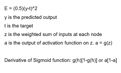
The 0.5 to Error function is added just to simplify the expression when we take the derivative of Squared Error. I encourage you to calculate the derivative of sigmoid function.
For simplicity, let’s just assume that we have only the weights and not the biases. So we need to determine how much the error will decrease when we tweak w and v.
First Layer
First, let’s calculate the differential with respect to V. We need to apply the mathematical concept of Chain Rule. I will try to break down the chain rule into it’s elementary components.
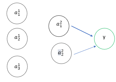
So those blue arrows are the weights we are going to change or update. Let’s think a bit logically here. When we change V, the weighted sum z changes. Since z changes, the output of the activation function changes. Since activation changes, the error E changes. Let’s put that in a Chain rule format.

Voila! There is our first equation.
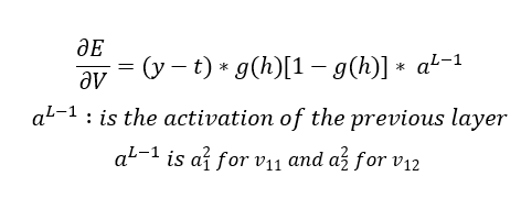
I am not going to solve the derivatives, that’s just simple differential calculus which I encourage you to solve on your own. The final equation looks like this
That completes the first step!
Second Layer
Now we need to determine how E varies when we vary W. As you can see, there is no direct connection between W and E and this is going to make things a bit more tougher.
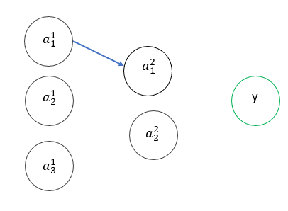
So if we set up a similar chain rule equation for E with respect to w11, we get

The equation in green is the equation for change of error with respect to W11.
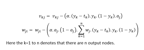
The generalized equations for weight update that is normally used in problem solving are,
So that brings us to the end of the backprop derivation. Honestly speaking, this can all be done with a single line of code in Keras and learning this might seem obsolete. But you might be required to solve problems in your exams which might require this working out. So that’s the only use for this as far as I know.
A Simple Example
So now consider the XOR problem. Let’s just run one epoch for one example. Let’s take x1=1, x2=0, y=0 and bias =1. The sigmoid activation function is used in the hidden layer and the output layer. The target is 1.
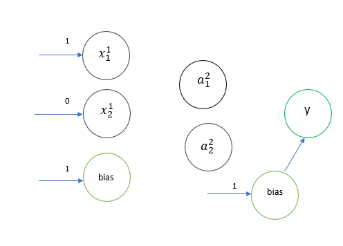
At the end of forward prop, we have the following,

Now let’s backprop!! This is the tougher part! I am using a learning rate of 0.3. The equations can be referred from above.

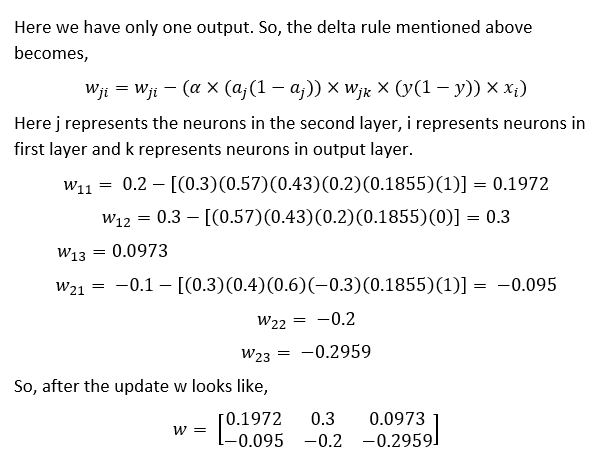
And w has also been updated!!!!!!
We have successfully completed one epoch of the training!!

This process is repeated till we manage to get the correct output.
I know that there was a lot of math in this post, but this is how the NN works and I have managed to justify one of my initial suppositions that “DL boils down to simple math“.
Next steps
In the next post, we will see the building of NN using Keras and use it to solve a problem.
See you in the next post.
References
I will mention some of the resources I looked at to understand these concepts.
- 3blue1brown
- Coding Train
- Backpropagation in Neural Networks
- Machine Learning- An algorithmic approach by Stephen Marshland
- Machine Learning by Tom Mitchell
I recommend you to go through the works of these people as they have explained these concepts better than me. I referred to these materials to get an understanding and I have shared that with you in this post. If you have referred to any other material and found it useful please share it in the comments section as it will be useful for others!
